05 — The render
| *Chaotic Curiosity | regolith series* |
Five chapters in, you have a trained model with two very different numbers. On synthetic data dr_1500 scores 0.852 rock-IoU — the best in the project. On real Apollo photographs (chapter 04) the same weights flood ~83% of the frame with false rock. The sim-to-real gap is named and measured, and it is wide. What you have not done yet is show the model working — in motion, on the kind of scene it was actually trained for.
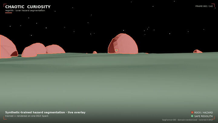
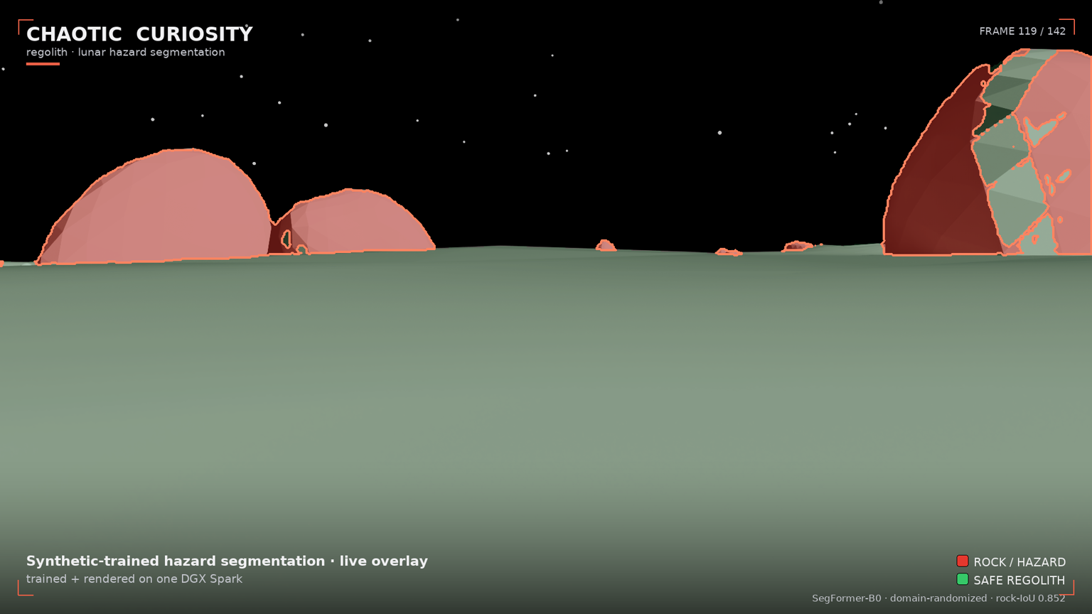
That is this chapter, and it comes with a warning attached. You will use NVIDIA Omniverse’s RTX renderer to fly a rover camera slowly into a boulder field — a low-sun scene with long raking shadows — and composite the trained hazard model’s predictions onto every frame in real time. Boulders glow red with a bright detection outline. Safe traversable ground goes green. Sky is untouched. The result is a rover’s-eye hazard HUD rendered cinematically at 1920 × 1080 and assembled into a flythrough — and it looks clean. That cleanliness is exactly the thing chapter 04 warned you not to trust: this scene is in-distribution, so the overlay flatters the model the same way the 0.852 synthetic score does. The render is the loop closing — synthetic data → trained model → per-frame inference → cinematic render, all on one 128 GB DGX Spark — and a live demonstration of why a beautiful synthetic result is not evidence of real-world readiness.
Why in-distribution — and why that is the honest choice
The scene was built to be in-distribution: every visual parameter — sun elevation, regolith albedo, rock count, camera height, field of view — falls inside the ranges train_dr.yaml used to generate the training set. The model has not literally seen this camera path or this rock layout, but it has seen this kind of scene.
That is a deliberate framing decision. When you want to demonstrate what a model can do at its best, you put it in the regime it was trained for. If you ran the overlay over the test_photoreal conditions (brighter sun, higher albedo, wider lenses) you would see more misfires — not because the model is broken, but because you moved it into known-harder territory. Chapter 04 already showed what out-of-distribution looks like. This chapter shows the in-distribution ceiling.
One cosmetic adjustment is applied: a --display-gain 0.78 is multiplied into the composite output only, to bring the brighter RTX render (auto-exposed to mean ~108) down toward the visual range of the training frames (mean ~82), so the overlay looks grounded rather than washed-out. The model runs inference on the original, unmodified pixels. The gain touches only what you see; it does not touch what the model sees. The predictions are real.
The scene: build_lunar_stage(seed=7, HERO_PARAMS)
The hero scene is procedurally generated with a fixed seed (7) and a hand-picked but in-distribution parameter set:
| Parameter | Value | Why |
|---|---|---|
| Sun elevation | 11° | Grazing — long raking shadows across the boulder field |
| Sun azimuth | 122° | Side-back; dome hole stays ~120° off-axis, safely outside the frustum |
| Sun intensity | 17 000 | High end of training range — high contrast |
| Regolith albedo | 0.19 | Mid-range, visually mid-gray |
| Terrain amplitude | 3.7 m | Slightly rugged |
| Rock count | ~95–125 far-field + 14 near boulders | Dense boulder field in the foreground |
| Camera height | 2.0 m | Nominal rover eye height |
| Camera FOV | 62° | Nominal lens |
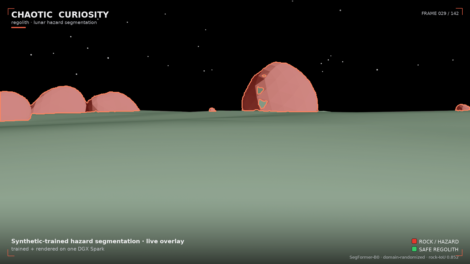
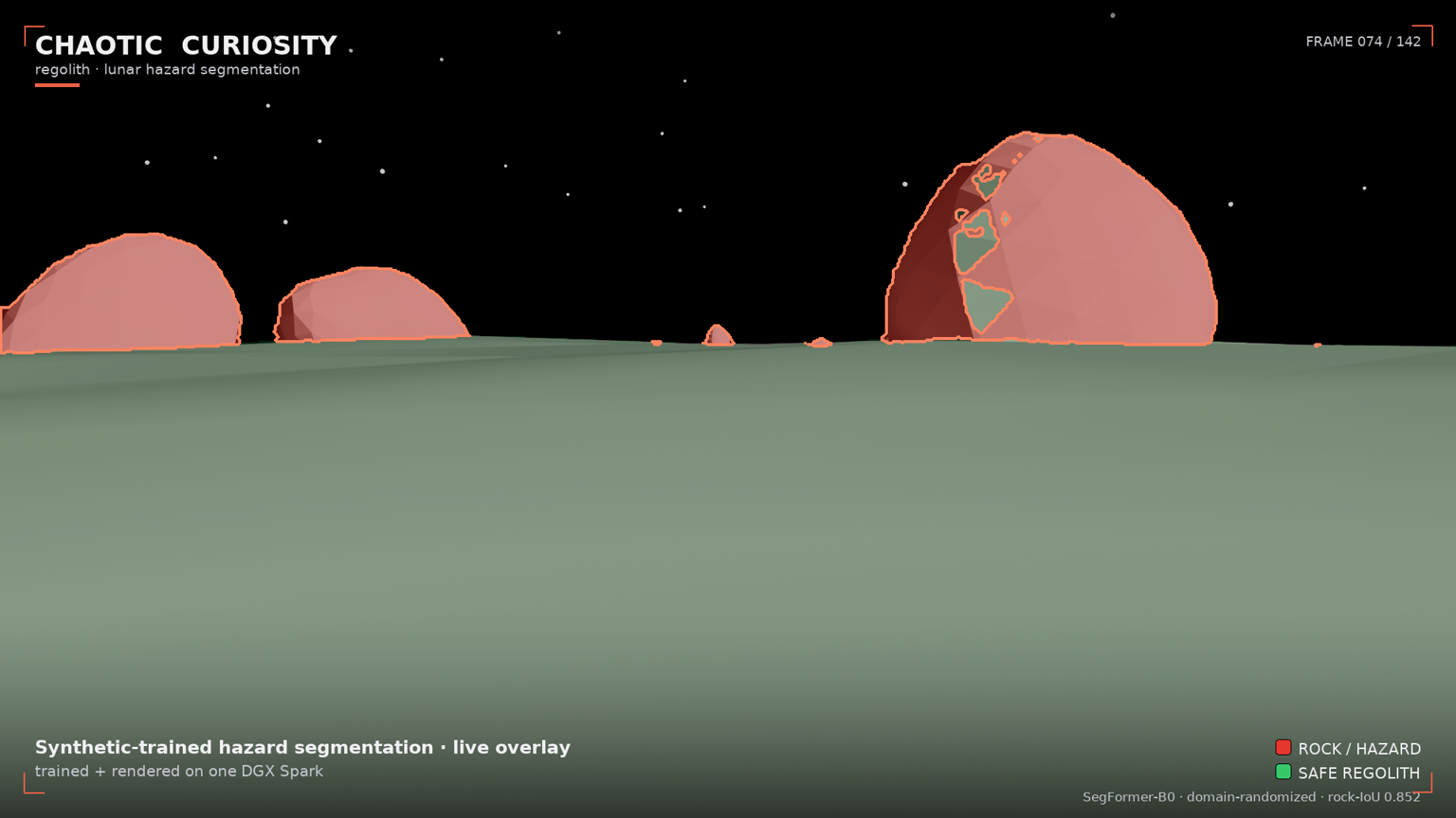
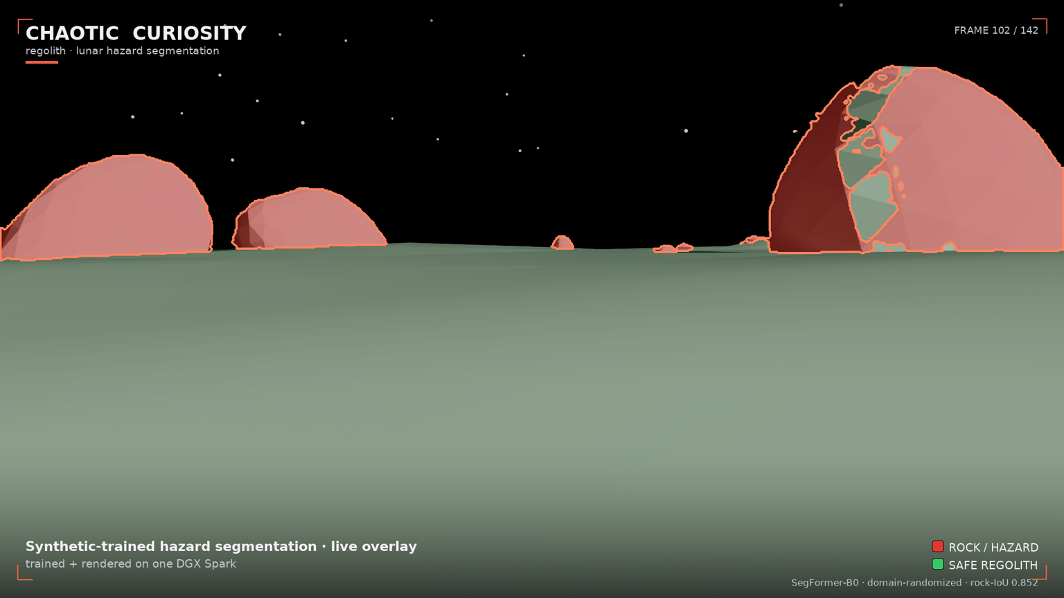
The camera follows a 252-pose flythrough path — a slow dolly forward (y: −95 → −63 m, closing ~32 m on the boulder field), a gentle lateral arc (±7 m), a slow yaw pan (+6° → −6°), an easing tilt (−1.5° → −3°), and a subtle vertical bob. The overall effect is a gradual approach toward the boulders, rocks growing in frame as the camera closes in. The model’s predicted rock fraction climbs from ~5% in the opening frames to ~9% in the final frames — an honest signal of the model registering more hazard as rocks fill the image.
RTX rendering: RayTracedLighting, 48 subframes, 1920 × 1080
The render uses RayTracedLighting — Omniverse’s full RTX path-tracing mode with global illumination, area shadows, and DLSS temporal accumulation. Key settings:
| Setting | Value |
|---|---|
| Resolution | 1920 × 1080 (full HD) |
| Mode | RayTracedLighting |
| RTX subframes | 48 (more accumulation passes per image, less path-tracing noise) |
| Wall-clock speed | ~2.4 s/frame warm |
| Total render time | ~10.4 min for 252 poses |
The pipeline has three stages, each self-contained:
- Stage A (render): Build the hero scene once, walk the 252-pose camera path inside a fresh Isaac Sim container, capture each frame from the
LdrColorannotator, skip-save until lit. Outputs: raw PNG frames inregolith_render/rgb/. - Stage B (overlay): Load each RGB frame in a PyTorch container, run
dr_1500/best.ptinference on each, composite the hazard visualization, add branding. Outputs: composited PNGs inregolith_render/overlay/. - Stage C (assemble): Call host
ffmpegto produce the full-res MP4, web preview MP4, hero stills, and the GIF. Host-side; no GPU needed.
The hard part: why BasicWriter wrote black frames
Here is the gotcha that consumed most of this session’s debugging time. It is worth understanding because it is a genuine trap in Omniverse RTX on this hardware.
BasicWriter — the standard Replicator output writer used in chapters 01 and 02 — writes all-black RGB frames. Not dark, not underexposed — exactly zero in every channel. The semantic segmentation masks rendered perfectly; only RGB was black. The first instinct (“is the scene set up wrong?”) is incorrect.
The root cause: BasicWriter captures at step time, synchronously, before NVIDIA’s DLSS temporal accumulation and auto-exposure pipeline have converged. The LdrColor buffer — the finished, post-processed color output — is still zero at capture time because the renderer has not had enough frames to complete its temporal integration. The semantic label buffer takes an entirely different, non-temporal path through the renderer, which is why semantics worked while RGB did not.
Confirmed via annotator probe: a BasicWriter frame read mean 0 at the same timestep that the LdrColor annotator read mean ~64 (fully lit).
The fix has two parts:
1. Read from the LdrColor annotator directly. Attach rep.annotators.get("LdrColor") to the render product, call .get_data() after each step, save the PNG yourself. This reads the output of the completed color pipeline — post-DLSS, post-exposure — rather than the raw step-time capture.
2. Drive convergence with real camera motion. A static camera, or a camera executing only tiny positional jitter, does not warm the temporal pipeline — verified experimentally. DLSS accumulation needs sustained translation and rotation. The render uses a single continuous capture pass with skip-save until mean pixel value > 50, numbering saved frames contiguously from the first lit one. No separate warmup loop; warmup happens as part of the hero approach path.
The warmup consumed approximately 108 of the 252 hero poses — the opening segment where the boulders are at their greatest distance. The 144 saved lit frames are the stable approach segment. Two more were dropped as edge cases (--skip-head 2), leaving 142 final frames. At 24 fps: 5.9 seconds of clean footage.
The hazard overlay
The overlay runs the same dr_1500/best.pt checkpoint from chapter 03 on each of the 142 lit frames. The inference path is identical to chapters 03 and 04:
- Input: rendered 1920 × 1080 PNG → downscaled to 1024 × 576 (16:9 aspect preserved), ImageNet-normalized
- SegFormer-B0 forward pass → logits at H/4 resolution → nearest-neighbor upsample to 1024 × 576 before argmax
- Predicted mask upsampled back to 1920 × 1080 (nearest-neighbor, preserving hard boundaries)
- Composite palette:
- rock — semi-transparent red tint + bright red outline drawn on the eroded inner edge of each detection, so the outline stays inside the predicted region rather than bleeding outward
- regolith — light green tint (lower opacity than rock — traversable ground stays visible through the highlight)
- sky — untouched
- Branding overlay: Chaotic Curiosity wordmark, scene caption, color legend, corner tick marks
The mean predicted rock fraction across all 142 frames is ~6.9%, consistent with a scene at the denser end of the in-distribution rock-fraction range (~1–8% in training). The fraction climbs from ~5% in the opening (boulders distant) to ~9% in the final frames (boulders close-in). The model is correctly tracking hazard proximity.
Why the overlay is clean — and the honest asterisk
The overlay looks coherent: tight outlines, green regolith floor, no stray rock bleeding into the sky. Three reasons, stated plainly:
In-distribution scene. The model trained on scenes that look exactly like this one — the same renderer, the same regolith heightfield, the same basalt boulders. The catastrophic failure from chapter 04 — flooding ~83% of a real frame with false rock, plus the rock-cloud in the sky — does not appear, because here the regolith is the synthetic regolith the model learned to tell apart from rock. On real film the soil carries the rough gray bumpy texture the model reads as rock; the renderer’s smooth heightfield does not. So the boundary that collapsed on real pixels holds perfectly here. This is the single most important caveat in the chapter: the overlay is clean because the ground is fake. The clean 0.852 synthetic score and this clean render are the same flattery, produced by the same in-distribution comfort — and chapter 04 is what happens when you remove it.
Inference on unmodified pixels. The --display-gain adjustment was applied after the fact, to the composite. The model’s input was the raw RTX LdrColor output — the same brightness regime as training frames, un-adjusted.
Boulder-field design. Fourteen near-field boulders close enough to produce solid large-area rock detections, against a clearly textured regolith floor and near-black sky. The scene was chosen to be legible, not to be the hardest possible case.
The clean overlay is a demonstration of the capability this series set out to build — a model that correctly identifies rocks when shown the kind of scene it trained on, shown cinematically. It is not a proof of real-world readiness, and after chapter 04 you should distrust it precisely because it is so clean. Chapter 04 is the reality check, and it showed not a gap but a flood. Both results are part of the honest record — and the gap between this beautiful render and that flooded Apollo frame is the whole point.
Reproduce
# Stage A — render RGB frames (Isaac Sim container)
# IMPORTANT: do NOT force-kill the container mid shader-compile.
# A stale .cache/ov/_cache.lock will cause the next container to hang at boot
# (SimulationApp never starts; GPU stays at 0%). Fix: rm the lock file and relaunch.
ssh spark "docker run -d --name isaac-render --entrypoint bash --gpus all --network=host \
  -e ACCEPT_EULA=Y -e PRIVACY_CONSENT=Y \
  -v /home/chaotic-curiosity/regolith:/workspace/regolith:rw \
  -v /home/chaotic-curiosity/regolith_render:/workspace/render_out:rw \
  -v /home/chaotic-curiosity/regolith_cache:/isaac-sim/.cache:rw \
  nvcr.io/nvidia/isaac-sim:6.0.0 -lc 'sleep infinity'"
ssh spark "docker exec isaac-render bash -lc 'cd /workspace/regolith && /isaac-sim/python.sh \
  render/render_predictions.py render --out /workspace/render_out --seed 7 --frames 252 \
  --width 1920 --height 1080 --renderer RayTracedLighting --subframes 48 \
  --prime-steps 8 --lit-threshold 50'"
ssh spark "docker rm -f isaac-render"

# Stage B — overlay predictions + branding (PyTorch container with transformers)
ssh spark "docker exec regolith-overlay bash -lc 'cd /workspace/regolith && python \
  render/render_predictions.py overlay --checkpoint outputs/runs_v2/dr_1500/best.pt \
  --rgb-dir /workspace/render_out/rgb --out /workspace/render_out/overlay \
  --display-gain 0.78 --skip-head 2'"

# Stage C — assemble MP4 + stills + preview (host ffmpeg — no GPU needed)
ssh spark "python3 /home/chaotic-curiosity/regolith/render/render_predictions.py assemble \
  --overlay-dir /home/chaotic-curiosity/regolith_render/overlay \
  --out /home/chaotic-curiosity/regolith_render --fps 24"
Outputs on the Spark:
regolith_render/regolith_flythrough.mp4— 1.23 MB, 1920 × 1080 H.264 faststart (git-excluded; published as a GitHub Release asset)regolith_render/rgb/— raw RTX framesregolith_render/overlay/— composited framesregolith_render/stills/— hero stills
Committed to docs/reports/assets/: render-hero-{1..4}.png, render-preview.mp4 (1280-wide, 0.18 MB), render-preview.gif (720-wide, 2.64 MB).
What you now understand
- RTX rendering in Omniverse uses
RayTracedLightingwithrt_subframesaccumulation for path-traced output; 48 subframes at 1920 × 1080 runs at ~2.4 s/frame on a DGX Spark. BasicWriterwrites black frames on this hardware because it reads theLdrColorbuffer before DLSS temporal accumulation and auto-exposure converge. Fix: attach anLdrColorannotator directly, drive convergence with sustained real camera motion, and skip-save frames below a brightness threshold.--display-gaintouches the composite only. The model sees the original pixels; the gain is cosmetic output adjustment. When you read “predictions are real,” this is what that means.- In-distribution vs out-of-distribution determines overlay quality more than model quality. The render demonstrates the flattering in-distribution ceiling (0.852); chapter 04 removed the comfort and measured the flood (~83% false rock on real soil). A clean synthetic overlay is not evidence of real-world readiness — it is the same in-distribution flattery the synthetic benchmark gives.
- The three-stage pipeline (render → overlay → assemble) keeps Isaac Sim, PyTorch, and ffmpeg in separate containers and host processes, avoiding dependency conflicts on the DGX.
- Never force-kill an Isaac container mid shader-compile — it leaves a stale
_cache.lockthat hangs the next container at boot.
The render is the loop closed: scene → dataset → trained model → cinematic inference, end to end on one machine. But it is also the most flattering view of the model in the entire series — the in-distribution best case, shown cinematically. Chapter 04 was the worst case, on real pixels. The two together raise the question the final chapter answers: we made the rocks realistic to improve this, and it made the real-world result worse — so what actually happened, and what is the lesson? Chapter 06 tells that story start to finish, with the before-and-after geometry side by side.
Continue to 06 — Rock fidelity: an evolution.