03 — Training the model
| *Chaotic Curiosity | regolith series* |
Chapter 02 produced three labeled datasets — rendered on the realistic basalt rocks of chapter 01: a 1,500-frame domain-randomized training set, a 750-frame no-DR control where only the appearance is frozen, and a 300-frame unseen-domain test set (test_photoreal). This chapter turns those pixels into a model — and then runs the experiment the whole series has been building toward: does domain randomization actually help, when you hold everything else equal?
The answer, measured: +0.046 rock-IoU at matched dataset size. That is a real gain — but it is smaller than the +0.099 the cruder first-build rocks produced, and the reason why is the seed of this whole series’ punchline. The realistic rocks lifted every score: the no-DR baseline jumped from 0.689 to 0.8025, so there was simply less gap left for domain randomization to close. This chapter explains what these numbers mean, how they were earned, and — just as importantly — why a higher synthetic score is about to mislead us.
What “training” means here: fine-tuning, not from scratch
You do not teach a network to see from nothing. That would need millions of images and weeks of compute. Instead you start from a model that already knows what edges, textures, and shapes look like, and you adjust it for your specific task. That adjustment is fine-tuning — continuing to train a model whose weights were already learned on a large general dataset, using a much smaller task-specific dataset.
The general knowledge comes from transfer learning: the idea that features learned on one task carry over to another. Our model’s visual “prior” comes from ImageNet — a 1.2-million-image classification dataset of everyday objects (dogs, cars, mushrooms). A network trained on ImageNet learns a hierarchy of reusable visual features in its early layers: oriented edges, then textures, then object parts. None of those are lunar, but edges are edges — the low-level machinery transfers cleanly to rock-vs-regolith boundaries. We keep that machinery and retrain the parts that decide “rock or not.”
The model is SegFormer — a semantic-segmentation architecture built on a Mix Transformer (MiT) backbone. We use its smallest variant, SegFormer-B0 (HuggingFace id nvidia/mit-b0), chosen in chapter 00’s plan for three reasons: it is fast to fine-tune on a 3-class problem, its hierarchical transformer reads multi-scale texture (pebble to boulder) better than a same-size convolutional backbone, and its low inference latency suits eventual onboard deployment.
One subtlety worth naming: we load the MiT encoder (the ImageNet-pretrained half that extracts features) but throw away SegFormer’s original output head and bolt on a fresh decode head sized for our 3 classes. The encoder starts smart; the head starts random and learns {regolith, rock, sky} from scratch on our data. In training/model.py, ignore_mismatched_sizes=True is exactly the flag that permits this transplant.
The rare-class problem: why the loss has to be weighted
A segmentation model is trained by a loss function — a number that measures how wrong each prediction is, which the optimizer drives downward. The default for classification is cross-entropy loss: per pixel, how much probability mass did the model put on the correct class?
Plain cross-entropy has a fatal flaw on this dataset. Recall from chapter 02 that rock — the hazard class, the entire point of the system — covers only 1–8% of pixels in a typical training frame; regolith and sky split the rest. A model minimizing average per-pixel loss discovers a cheap shortcut: predict “regolith” or “sky” almost everywhere, eat the small penalty on the rare rock pixels, and still post a low average loss. It would score high on overall accuracy and detect no hazards. That is the worst possible failure mode for a rover.
The fix is class-weighted cross-entropy: multiply each class’s contribution to the loss by a weight inversely proportional to how common it is, so a mistake on a rare rock pixel costs far more than a mistake on common regolith. training/train.py computes these weights from the actual pixel counts of each training split (inverse frequency, normalized to sum to 3). The result for every run lands at roughly:
| Class | Pixel share | Loss weight |
|---|---|---|
| regolith | dominant | ~0.20 |
| rock | 1–8% | ~2.59 |
| sky | dominant | ~0.20 |
A rock pixel carries about 13× the loss weight of a regolith pixel. That is what forces the model to take the hazard class seriously instead of averaging it away.
Two more pieces complete the loss: pixels labeled 255 (the ignore index — background or unlabeled, see chapter 01) are excluded from the loss entirely, and rock-IoU (not overall accuracy, not mean-IoU) is the metric used to pick the best checkpoint. IoU — intersection over union — measures predicted-rock pixels that are truly rock, divided by the union of predicted and true rock. It is the honest score for a rare class: predicting “regolith everywhere” scores an IoU of 0 on rock, no matter how high the overall accuracy. We save the checkpoint with the highest validation rock-IoU and report that number.
The training configuration
Every run is identical except for the training data — that is the whole design. The shared recipe:
| Setting | Value | Why |
|---|---|---|
| Model | SegFormer-B0 (nvidia/mit-b0) |
Smallest SegFormer; ImageNet MiT encoder + fresh 3-class head |
| Loss | Class-weighted CE, ignore_index=255 |
Rock up-weighted ~13× (above) |
| Optimizer | AdamW, peak lr 6e-5 | SegFormer paper’s fine-tuning rate |
| LR schedule | Cosine decay to 1e-7 | Smooth anneal over the run |
| Batch size | 8 | Fits comfortably in the Spark’s unified memory |
| Validation split | test_photoreal |
Unseen-domain synthetic — the generalization probe |
| Early stopping | patience 8 on val rock-IoU | Stop once it stops improving (max 40 epochs) |
| Seed | 0 | Same initialization and data order across runs |
| Hardware | DGX Spark (GB10), NGC pytorch:26.03-py3, transformers |
~16–31 s/epoch |
Using test_photoreal as the validation set is deliberate: we are not measuring how well each model fits its own training distribution (every model fits its own data well — see the overfitting evidence below). We are measuring how well it generalizes to a domain it never trained on. That is the number that predicts real-world behavior.
The honest ablation: hold dataset size constant
Here is where most “domain randomization works!” claims quietly cheat. The deployed DR set has 1,500 frames; the no-DR control has 750. Compare those two directly and you have changed two things at once — the randomization and twice the data. Any improvement is confounded: you cannot tell how much came from DR and how much came from simply training on more images.
So we run a size-matched ablation — the controlled experiment that isolates the variable you care about. Three runs:
nodr_750— the no-DR control. 750 frames, appearance frozen.dr_750— domain-randomized, but truncated to the same 750 frames. On the Spark this split is literally the first 750 frames of the 1,500-frame DR set, symlinked — same generation, same seed lineage, just cut to match the control’s count.dr_1500— the full deployed DR set, 1,500 frames.
Now the comparisons separate cleanly:
dr_750vsnodr_750isolates domain randomization — identical size (750), identical content distribution (chapter 02 showed both vary rock layout and terrain the same way); the only difference is whether appearance was randomized. This is the headline.dr_1500vsdr_750isolates dataset size — identical method (DR), 750 → 1,500 frames. This is the secondary, “more data” effect.
Comparing 1,500-vs-750 would have inflated the apparent DR benefit by smuggling in the data-size gain. The size-matched design refuses that shortcut.
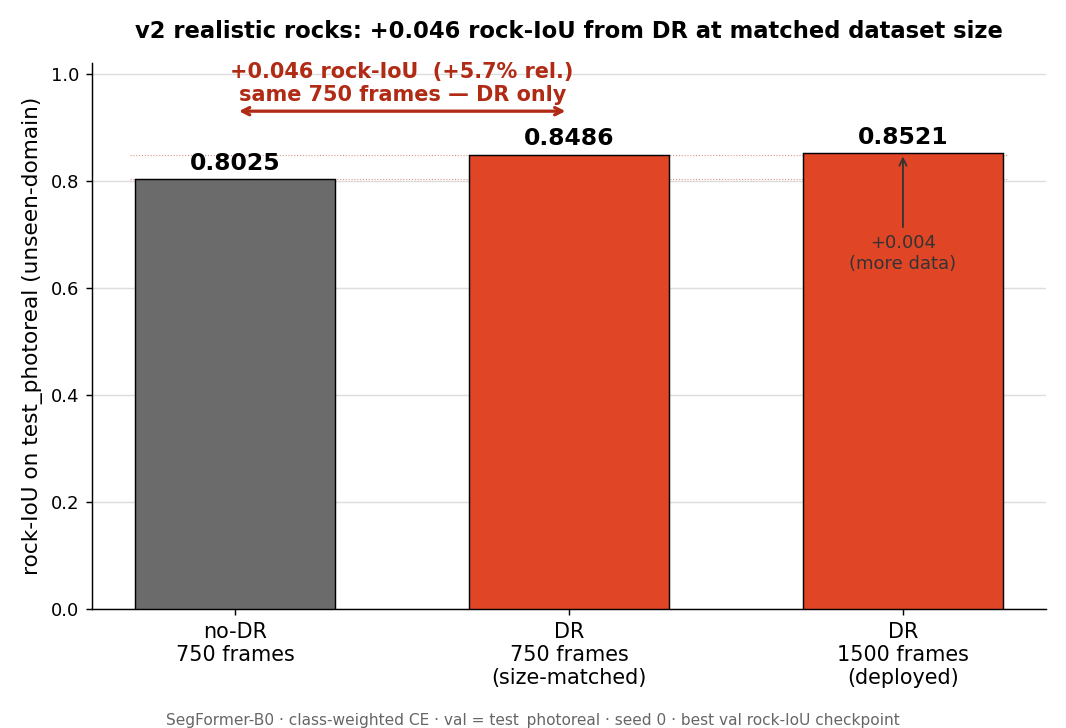
Results
All three runs, best validation checkpoint on test_photoreal:
| Run | Frames | DR? | rock-IoU | best epoch |
|---|---|---|---|---|
nodr_750 |
750 | no | 0.8025 | 18 |
dr_750 |
750 | yes | 0.8486 | 19 |
dr_1500 |
1,500 | yes | 0.8521 | 13 |
For the deployed dr_1500 checkpoint, the full per-class breakdown is regolith 0.9556 / rock 0.8521 / sky 0.9730, mIoU 0.9269.
Read the two effects straight off the table:
- Domain randomization, size-matched: rock-IoU 0.8025 → 0.8486 = +0.046 absolute (+5.7% relative), with dataset size held fixed at 750. Pure DR.
- More data, DR held fixed: rock-IoU 0.8486 → 0.8521 = +0.004 going from 750 to 1,500 frames. Effectively flat — the curve has saturated. Doubling the data bought almost nothing.
Two things changed from the cruder first build, and both matter. First, every number is higher: the realistic basalt geometry is simply easier to learn and to generalize from, lifting the no-DR baseline from 0.689 all the way to 0.8025. Second — and this is the consequence — the DR gain shrank, from +0.099 to +0.046, and the more-data gain all but vanished (+0.004). When the floor rises that far, there is less room left above it for either lever to add. Regolith (0.9556) and sky (0.9730) are at ceiling; what little headroom remains is in rock, the one class that matters for not destroying a wheel.
The full numeric table — including the v1-vs-v2 comparison and the independent verification pass — is committed alongside the figures at assets/ablation-results.json. The dr_1500 global IoU was re-derived in a fresh inference pass over all 300 test frames straight from the saved checkpoint — rock-IoU 0.8520, mIoU 0.9269 — matching the training-time number (0.8521) to three decimals, so the inference path is faithful.
Why the DR gain shrank: the floor came up
The mechanism is the same one domain randomization always fights — overfitting to a frozen appearance — but the realistic rocks changed the size of the prize.
In the cruder first build, the no-DR model had a soft target to memorize: smooth, low-poly rocks under one fixed lighting were easy to overfit and brittle to generalize, so the no-DR baseline languished at 0.689 and DR’s anti-memorization pressure bought a full +0.099. The realistic basalt rocks are a richer, more varied signal in their own geometry — every boulder is a distinct eroded shape — so even a no-DR model trained on them generalizes much better to the unseen-domain test set (0.689 → 0.8025). Realistic geometry, it turns out, does part of the job domain randomization used to do alone.
That is why the size-matched DR gain fell to +0.046: there was less brittleness left to fix. And it is why more data saturated almost immediately (+0.004 from 750 → 1,500) — once the model has learned generalizable rock-ness from realistic shapes, additional frames of the same kind add little. Both observations point the same way: fidelity and domain randomization are partly redundant levers. Raise one and the other has less to contribute.
Read at face value, this is good news, and the table says so: realistic rocks plus DR give the highest synthetic rock-IoU this project has produced, 0.8521. If the story ended at the synthetic benchmark, “we made the rocks photoreal and the number went up” would be the headline.
The story does not end at the synthetic benchmark.
The caveat that matters: this is still synthetic
Read the headline precisely. The +0.046 gain — and the 0.8521 ceiling it sits under — is measured on test_photoreal, a synthetic, held-out, unseen-domain split. Chapter 02 built it specifically to sit outside the training distribution: brighter sun (42°–70° elevation vs 5°–40°), higher albedo, rougher terrain, wider lenses, bigger and fewer rocks. So this is a real and demanding generalization test — the model predicts on lighting, materials, and geometry it never trained on.
But test_photoreal is still rendered by the same simulator that made the training data. It is synthetic → synthetic transfer. It is not yet the question the whole series exists to answer: does any of this survive contact with a real lunar photograph, taken by a real camera, of real regolith, under a real sun? That is the sim-to-real gap, and it is measured — honestly, with real imagery — in chapter 04.
And here is the trap we are walking into with our eyes open. We made the rocks photoreal; the synthetic score rose to 0.8521, the best in the project. The natural inference — better fidelity, better number, therefore better model — is the one chapter 04 is about to break. The realistic rocks are rough, gray, and bumpy. So is real lunar regolith at photographic resolution. A model trained to call “rough gray bumpy texture” rock learned something that scores beautifully on synthetic rocks and catastrophically over-fires on real soil. The 0.8521 is real. It is also about to mislead us. Turn the page.
Reproduce
All three runs, on the Spark, inside the training container (regolith-train, NGC pytorch:26.03-py3 with transformers). Datasets at /workspace/datasets/, code mounted at /workspace/regolith:
# 0. Size-matched DR split = first 750 frames of train_dr, symlinked
ssh spark "mkdir -p /home/chaotic-curiosity/regolith_data/train_dr_750/{rgb,mask}
  cd /home/chaotic-curiosity/regolith_data/train_dr_750
  for i in \$(seq -f '%05g' 0 749); do
    ln -sf ../../train_dr/rgb/rgb_\$i.png  rgb/rgb_\$i.png
    ln -sf ../../train_dr/mask/mask_\$i.png mask/mask_\$i.png
  done"

# 1. no-DR control (750)
ssh spark "docker exec regolith-train bash -lc \
  'cd /workspace/regolith && python training/train.py \
     --train-split /workspace/datasets/train_nodr \
     --val-split   /workspace/datasets/test_photoreal \
     --epochs 40 --lr 6e-5 --batch 8 --seed 0 --patience 8 \
     --out /workspace/regolith/outputs/runs_v2/nodr_750'"

# 2. DR, size-matched (750)
ssh spark "docker exec regolith-train bash -lc \
  'cd /workspace/regolith && python training/train.py \
     --train-split /workspace/datasets/train_dr_750 \
     --val-split   /workspace/datasets/test_photoreal \
     --epochs 40 --lr 6e-5 --batch 8 --seed 0 --patience 8 \
     --out /workspace/regolith/outputs/runs_v2/dr_750'"

# 3. DR, full deployed set (1500)
ssh spark "docker exec regolith-train bash -lc \
  'cd /workspace/regolith && python training/train.py \
     --train-split /workspace/datasets/train_dr \
     --val-split   /workspace/datasets/test_photoreal \
     --epochs 40 --lr 6e-5 --batch 8 --seed 0 --patience 8 \
     --out /workspace/regolith/outputs/runs_v2/dr_1500'"
Each run writes best.pt, metrics.jsonl (per-epoch curves), and summary.json (final numbers) to its output dir. Checkpoints stay on the Spark — they are heavy binaries, excluded from git. The figures and the results table in docs/reports/assets/ are the committed artifacts.
What you now understand
- Fine-tuning adapts a model that already learned general vision via transfer learning from ImageNet; we keep SegFormer-B0’s MiT encoder and train a fresh 3-class decode head.
- The rock class is 1–8% of pixels, so plain cross-entropy would ignore it; class-weighted cross-entropy up-weights rock ~13× and rock-IoU (not accuracy) selects the best checkpoint.
- The size-matched ablation (
dr_750vsnodr_750, both 750 frames) isolates domain randomization from dataset size — the honest comparison that 1500-vs-750 would have confounded. - On the realistic rocks, domain randomization adds +0.046 rock-IoU (+5.7%) at matched size (0.8025 → 0.8486); doubling the data on top adds only +0.004 (0.8486 → 0.8521) — the curve has saturated. The deployed
dr_1500ceiling is 0.8521 (regolith 0.9556 / rock 0.8521 / sky 0.9730). - The DR gain is smaller than the +0.099 the cruder rocks gave, because realistic geometry raised the no-DR baseline from 0.689 to 0.8025. Fidelity and domain randomization are partly redundant levers — raise one and the other has less left to add.
- This is still a synthetic unseen-domain test, and the higher synthetic score is about to be a trap: a model that learned “rough gray bumpy = rock” scores beautifully on photoreal synthetic rocks and is primed to over-fire on real regolith. The real sim-to-real gap is chapter 04.
Continue to 04 — Sim-to-real.