Chapter 07 — Proving It’s Real
Chapter 06 ended with a confident walking robot — torso upright, weight shifting smoothly, arms swinging in rough counterbalance to its legs. The numbers looked good: mean reward 50.5, mean episode length 995. But you only have one run. How do you know it wasn’t luck? And how do you know the numbers are measuring what you think they are? This chapter answers both questions.
Part III continues: stress-testing the first skill
Chapter 06 showed you the gait that emerged. This chapter stress-tests it. Two moves: first, run the same training from scratch and check whether you get the same curve — that is the reproducibility argument. Second, pull the total reward apart into its individual components and watch each one develop separately — that is the reward-term breakdown. Along the way this chapter formally introduces termination: the mechanism that decides when an episode ends early, and why it matters more than it might seem.
One run is encouraging. Two runs are evidence.
Here is the honest situation after Chapter 06: you have a beautiful reward curve and a robot that walks. You have no idea whether that curve will appear again if you restart from zero, or whether you got lucky with a particular set of random starting weights. Training involves randomness at every stage — the random initial weights of the policy network, the random episode resets, the random order in which the simulator samples environment states. Any of those could cause a run to succeed or fail for reasons that have nothing to do with the recipe.
Reproducibility means: if you run the same recipe again, with the same configuration, you get the same result. Not byte-for-byte identical numbers — that would require eliminating all GPU non-determinism, which is essentially impossible in practice — but the same shape of curve, the same phases, the same final trajectory. If two independent runs both produce an S-curve with the same flat floor, the same sharp climb in roughly the same window, and a similar final reward level, you have strong evidence the algorithm is doing something real and consistent. If the second run fails or diverges wildly, the first run might have been a fluke.
The random seed
One specific source of randomness is the seed — a starting number that initializes the pseudo-random number generator used throughout training. The policy’s starting weights, the order of episode resets, the initial simulator states: all of these draw from a random stream that begins with the seed. If you run with the same seed, you get the same stream of random draws. If you change the seed, you get a different-but-statistically-equivalent stream.
Think of the seed like the shuffle you apply to a deck of cards before a card game. A fixed seed always shuffles the deck the same way. A different seed gives a different shuffle, but the same game rules still apply. Two runs with different seeds are genuinely independent — they experienced different random starting conditions — but if both produce the same outcome, the outcome is not a product of luck.
For the reproduction run, we used seed 42 — the framework’s default, which was also the baseline run’s seed. This is important: it means the two curves are not completely independent draws (they started from the same random conditions), but they were run at different times, on different hardware states, with separate CUDA execution streams. The agreement between them confirms the training pipeline is stable — there is no hidden run-to-run corruption that makes results unrepeatable under the same configuration. It does not prove robustness to initialization. Testing robustness to initialization — showing the same result emerges from genuinely different random starting weights — requires running with a different seed, and that is flagged here as a further experiment, not run in this chapter. Here, the goal is the simpler check: does the same recipe reproduce?
The reproduction run: the exact command
The fresh run used the identical recipe as the original baseline, launched inside the mjlab-dev container on the DGX Spark:
ssh spark "docker exec mjlab-dev bash -lc '
  cd /workspace/mjlab && \
  MUJOCO_GL=egl CUDA_VISIBLE_DEVICES=0 \
    python -u -m mjlab.scripts.train Mjlab-Velocity-Flat-Unitree-G1 \
    --env.scene.num-envs 2048 \
    --agent.max-iterations 1500 \
    --agent.run-name arc-control
'"
Every flag explained:
MUJOCO_GL=egl— tells the physics simulator to use the GPU’s offscreen rendering backend rather than a display window, which is required on a headless server.CUDA_VISIBLE_DEVICES=0— restricts the run to the first GPU, keeping the machine’s other resources free.Mjlab-Velocity-Flat-Unitree-G1— the task: a Unitree G1 humanoid on flat terrain, commanded to match a target velocity. This is the velocity tracking task introduced in Chapter 06.--env.scene.num-envs 2048— run 2,048 copies of the robot in parallel. More parallel environments means more experience collected per PPO update, which generally means faster learning.--agent.max-iterations 1500— stop after 1,500 iterations. The original baseline ran to 2,050 — we stopped short to confirm reproducibility without duplicating the full compute cost.--agent.run-name arc-control— a label for this run in the experiment logs, to distinguish it from the original.
No explicit --agent.seed 42 flag is needed: 42 is the framework default, and both runs used it. The run took roughly 26 minutes — about 1 second per iteration — on a single NVIDIA GB10 GPU.
Before launching, three co-tenant services sharing the machine’s memory were stopped. The Spark uses unified memory — the GPU and CPU share one physical pool of RAM. When that pool fills, the machine does not throw a clean “out of memory” error; it starts swapping data to storage and can spiral into a hard reboot, destroying the training run entirely. The workload used roughly 13 GB against ~110 GB available once the co-tenants were quiesced, so swap was never engaged.
The result: the curves match
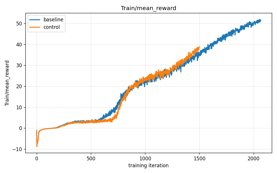
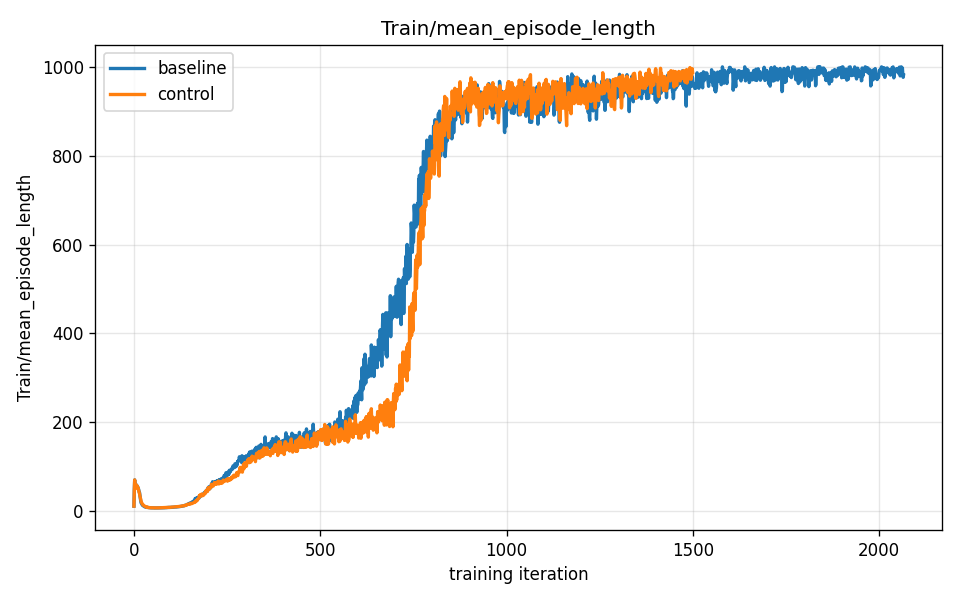
Both plots overlay the original baseline (blue) and the fresh control run (orange) on the same axes.
The curves nearly overlap through iteration 1,500. Both start near zero. Both climb sharply between roughly iterations 700 and 900 — the “aha” moment described in Chapter 05, where the policy first learns to stay upright long enough to earn velocity-tracking reward. Both flatten into the same refinement phase afterward.
A closer look at specific checkpoints:
| Iteration | Baseline reward | Control reward | Baseline episode length | Control episode length |
|---|---|---|---|---|
| 500 | 3.3 | 2.9 | 173 | 162 |
| 900 | 21.3 | 19.5 | 962 | 926 |
| 1,400 | 31.5 | 36.0 | 925 | 996 |
| 1,500 | — | 38.4 | — | 988 |
| 2,050 | 50.5 | — | 995 | — |
The baseline ran longer (to 2,050 iterations, reaching a final reward of 50.5). The control, stopped at 1,500, reached 38.4 — consistent with where the baseline was at that same point in its own run.
On the small differences
At iteration 1,400 the control (36.0) is slightly ahead of the baseline (31.5), before converging again. Don’t read too much into which run is momentarily higher at any single checkpoint. In the refinement phase, small run-to-run differences are expected and honest: they come from GPU non-determinism (the order in which thousands of floating-point additions are accumulated on the GPU can shift subtly between runs, even with the same seed) and from slightly different random episode resets. If the two curves were perfectly identical, that would actually be suspicious — it would suggest the runs were not truly independent.
What matters for reproducibility is the shape: the same slow start, the same sharp climb in the same window, the same refinement trajectory. Both runs show this. The result is real.
Insight: reproducibility is not about identical numbers — it is about consistent shape. A run-to-run difference of a few reward points is noise in the training process. Two runs that both show the same S-curve phases, in the same iteration windows, with similar endpoints, are telling you the same story about what the algorithm is doing. The story is reproducible. The exact numbers are not, and they don’t need to be.
Pulling the reward apart: the reward-term breakdown
The total reward in the plots above is a single number per iteration. But the total reward is the sum of several reward terms (introduced in Chapter 06), each scoring a different aspect of behavior. When the total goes up, you cannot tell from a single number which term drove the improvement: did the robot get better at tracking speed, better at staying upright, better at taking clean steps? The reward-term breakdown answers that by plotting each component separately.
The four plots below come from the control run. Raw scalar data is in assets/control_scalars.csv if you want to inspect the numbers directly.
Term 1: Track linear velocity — the primary job
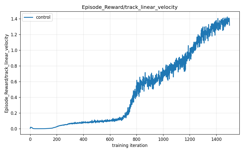
This term scores how closely the robot’s actual forward speed matches the commanded speed. It is computed by comparing the commanded velocity to the measured velocity at each timestep, and giving a higher score when the difference is small. This is the largest contributor to total reward — the “please go forward at 1 m/s” signal. Early in training it sits near zero, because the robot cannot walk at all. It rises as the robot learns to track the command, and the shape of its curve closely mirrors the shape of the total reward curve. If you only had one term to watch, this would be it.
track_lin_vel score ≈ exp(−gap² / std²)
Where gap is the difference between commanded and actual forward speed, and std is a tolerance parameter set by the designer. A perfect match (gap = 0) gives a score of 1. As the gap grows, the score drops toward zero exponentially. The idea is: being close is rewarded; being far away earns almost nothing.
Term 2: Upright — don’t tip over
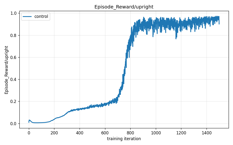
This term scores how vertical the robot’s torso is. A perfectly upright torso earns full points; leaning costs points. The curve rises quickly — relatively early in training, the robot learns that tipping over ends the episode (more on this shortly) and therefore learns to stay upright. It then stays high throughout. Upright posture is not something the robot discovers late; it is one of the first things it figures out, because survival depends on it.
Term 3: Air time — take real steps
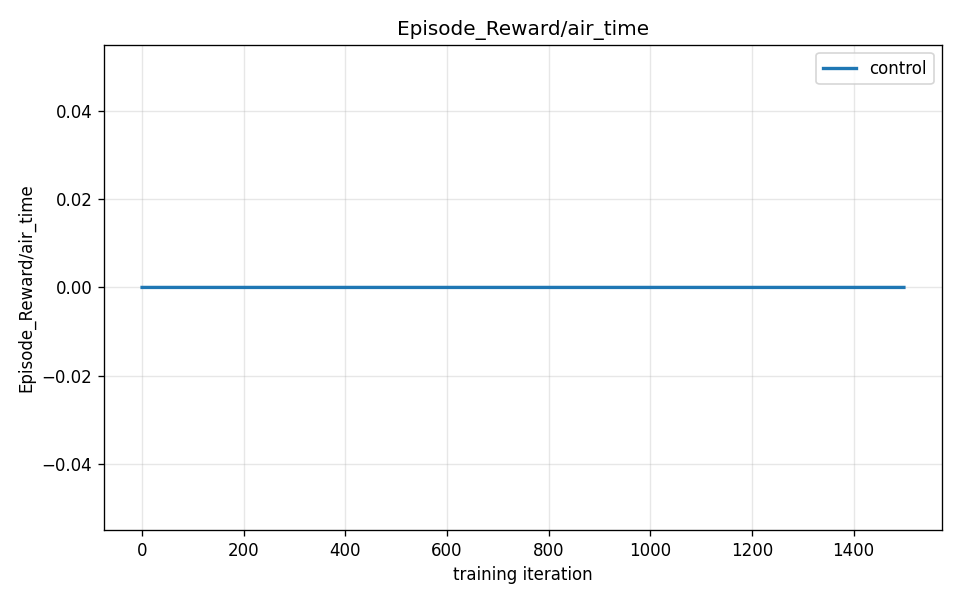
This is a gait-shaping term. It gives a small bonus each time a foot is genuinely in the air — not sliding along the ground or barely lifting, but fully airborne for a moment. Without a term like this, the optimizer tends to discover that dragging feet forward is a cheap way to move without truly stepping: you can match a forward velocity by shuffling without ever getting a foot off the ground. Air time explicitly rewards picking feet up.
The curve rises gradually and reaches a lower peak than track_lin_vel or upright — this is the expected pattern for a relatively small-weight shaping term. Its voice in the choir is quieter, but without it the gait character changes noticeably (as Chapter 09 will show in a different context).
Term 4: Action rate — smooth, not jerky
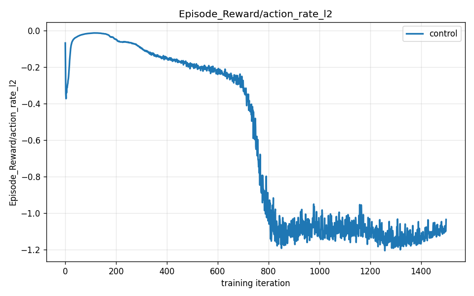
This is a penalty: it subtracts from the total reward in proportion to how rapidly the motor commands change from one timestep to the next. Large step-to-step changes in joint targets are penalized; smooth, gradual changes earn less penalty. Notice the curve is negative throughout — that is correct for a penalty term. As training progresses, the magnitude decreases (the curve drifts toward zero), meaning the policy is producing progressively smoother motor commands over time.
The intuition: jerky, rapidly oscillating commands are hard on real actuators. They also tend to produce unstable motion. The penalty is not about aesthetics — it is about keeping the robot in a regime where its commands are coherent and physically realizable.
What the breakdown reveals
Together, the four curves tell a story the total-reward plot obscures:
uprightrises first — surviving the episode is the prerequisite for everything else.track_lin_velhas the sharpest climb and the highest plateau — this is the main job, and once balance is established, the optimizer focuses here.air_timerises more slowly — gait refinement is a secondary improvement that emerges after basic locomotion is established.action_rate_l2starts strongly negative and steadily improves — smoothing out the motor commands is a refinement that takes most of the training run.
There are additional terms beyond these four — pose, foot_clearance, foot_slip, soft_landing, and others — each contributing smaller pieces to the total. The four above are highlighted because they most directly explain why the gait looks the way it does. The complete numerical record, including all terms across all iterations, is in assets/control_scalars.csv.
Insight: the total reward is a summary; the breakdown is the diagnosis. A rising total reward tells you learning is progressing. A per-term breakdown tells you what the robot is actually learning to do. Two runs with the same total reward could have very different term profiles — one robot might be excellent at speed tracking and terrible at smooth motion, while another has the opposite pattern. Never trust the total alone. The term breakdown is the first tool in your debugging toolkit, and you will use it repeatedly in the chapters ahead.
Termination: when and why episodes end early
Every episode ends in one of two ways.
Time-out: the robot survived the full episode duration — 1,000 timesteps, roughly 20 simulated seconds — without triggering any failure condition. This is success. The episode ends because the clock ran out, not because anything went wrong.
Termination: a condition was triggered that the environment considers a failure, and the episode was cut short. The robot earns no more reward after termination, and the simulator resets to a fresh starting state.
A termination is a condition that ends the episode early when the robot does something that signals unrecoverable failure. In the walking task, the primary termination is simple: if the robot’s torso drops below a height threshold, the episode ends. The exact threshold is set by the environment configuration; in the baseline walking task, it catches falls that would be irrecoverable in a real system — the robot’s body touching the ground, or nearly so. There is no mechanism to get back up, so there is no point continuing an episode where the robot has already collapsed.
Termination matters for learning in two ways.
Shorter episodes mean sparser rewards. A robot that terminates at timestep 50 earns reward for 50 timesteps; a robot that survives to timestep 1,000 earns reward for 1,000 timesteps. The policy that survives longer has much more experience to learn from per episode. This is exactly the feedback loop described in Chapter 05: once the robot learns to avoid early termination, it gets dramatically richer signal, which lets it improve faster, which lets it survive longer. The episode-length plot tracks this directly — early in training it sits at 162 steps (most runs ending in termination), then shoots to 988 steps (almost every run timing out) as the policy crosses the balance threshold.
Termination creates a sharp behavioral signal. Without termination, the robot could learn to stumble along in a half-fallen state, earning small rewards while never fully committing to upright walking. Termination makes falling unambiguously bad: it ends the episode, cutting off all future reward. This sharpens the learning signal — staying upright is not just better, it is a prerequisite for earning anything at all.
Think of termination as the equivalent of “game over” in a video game. The game ending is not the objective; the score is the objective. But “game over” shapes behavior powerfully, because it is the boundary that separates runs that can accumulate score from runs that cannot.
Early in the control run — iteration 500, mean episode length 162 — almost every episode ends in termination. The robot falls almost immediately. By the end — iteration 1,500, mean episode length 988 — almost every episode times out. The robot has learned, above all else, to not trigger the termination condition. The rising episode-length curve is the most direct signature of the termination learning effect.
Insight: termination shapes behavior before rewards do. In the walking task, the clearest behavioral shift is not the discovery of forward motion — it is the discovery of not falling. The robot learns to avoid termination before it learns to track velocity, because the termination penalty (losing all future reward) dominates the gradient signal in the earliest phase of training. This is why the
uprightterm rises first in the breakdown: upright posture is what keeps the episode alive, and surviving the episode is more valuable than anything else at that stage.
What the per-term plots confirm about the claim
Now you can close the loop on “is this real.”
The total reward curves matched across two independent runs — that is reproducibility. But “the total reward is high” could, in principle, reflect some unexpected gaming of the reward signal rather than actual walking behavior. The term breakdown rules this out: the term profiles tell a coherent mechanical story. upright rises first (the robot learns to survive), then track_lin_vel climbs sharply (the robot learns its primary job), then air_time and action_rate_l2 refine together (the gait improves in quality). There is no term that shoots up anomalously while others stay flat in a way that would suggest the policy found a shortcut that satisfies the number but not the behavior.
This combination — curves that reproduce, terms that tell a coherent story — is what establishes “this is real.” Any one of those checks can be fooled; the combination is much harder to fool.
There will be runs later in this series where one check passes and the other fails. When they diverge, something interesting is happening. Chapter 09 shows a case where the reward rises but the per-term breakdown reveals the policy found an unexpected shortcut. Having both checks in your toolkit is what lets you catch it.
What you now understand
Reproducibility: running the same training recipe from scratch and getting the same shape of curve — not the same numbers, but the same phases in the same windows with a comparable endpoint — is strong evidence the result is not noise. The seed controls the initial random state; using the same seed with the same config gives you the closest possible reproduction. Using a different seed tests robustness to initialization.
Reward-term breakdown: inspecting each reward component individually reveals what the policy has actually learned to optimize. A rising total reward is necessary but not sufficient; the term profiles tell you whether the improvement is mechanically coherent. Four terms drove the walking behavior: track_lin_vel (the primary job), upright (staying alive), air_time (taking genuine steps), and action_rate_l2 (smoothing the commands). The raw scalar data is in assets/control_scalars.csv.
Termination: a condition — such as the robot’s torso falling below a height threshold — that ends the episode early. Termination shapes behavior powerfully: it makes failure unambiguous and creates a sharp incentive to stay upright. The episode-length metric is the most visible signature of termination learning: when it rises sharply, the robot has learned to avoid the conditions that trigger early episode endings.
In Chapter 08, you will start pulling the knobs — changing reward weights and watching how the gait and curves shift. Now that you can read both the total reward and the term breakdown, you will be able to tell not just whether a change made the number go up, but what specifically the robot changed about its behavior to earn the higher score. And you will encounter the first case where a higher number does not mean a better robot.
Continue to Chapter 08 — Turning the Knobs.